Wasserstein GAN

v. 1.0

While reading the Wasserstein GAN paper I decided that the best way to understand it is to code it. This is a quick overview of the paper itself and is followed by the actual code in Keras.

GAN?

GAN, or Generative Adversarial Network is a type of generative model – a model that looks at the training data drawn from a certain distribution and tries to estimate that distribution. New samples obtained from such model “look” alike original training samples. Some generative models only learn the parameters of training data distribution, some only able to draw samples from it, some allow both.

Many types of generative models exist: Fully Visible Belief Networks, Variational Autoencoders, Boltzmann Machine, Generative Stochastic Networks, PixelRNNs, etc. They differ in a way they represent or approximate the density of the training data. Some construct it explicitly, some just provide ways to interact with it – like generating samples. GANs fall into latter category. Most generative models learn by maximum likelihood estimation principle – by choosing the parameters of the model in such a way that it assigns maximum probability (“likelihood”) to training data.

GANs work by playing a game between two components: Generator (G) and Discriminator (D) (both usually represented by neural nets). Generator takes a random noise as input and tries to produce samples in such a way that Discriminator is unable to determine if they come from training data or Generator. Discriminator learns in a supervised manner by looking at real and generated samples and labels telling where those samples came from. In some sense, Discriminator component replaces the fixed loss function and tries to learn one that is relevant for the distribution from which the training data comes.

Wasserstein GAN?

In essence the goal of any generative model is to minimize the difference (divergence) between real data and model (learned) distributions. However in traditional GAN D doesn’t provide enough information to estimate this distance when real and model distributions do not overlap enough – which leads to weak signal for G (especially in the beginning of the training) and general instability.

Wasserstein GAN adds few tricks to allow D to approximate Wasserstein (aka Earth Mover’s) distance between real and model distributions. Wasserstein distance roughly tells “how much work is needed to be done for one distribution to be adjusted to match another” and is remarkable in a way that it is defined even for non-overlapping distributions.

For D to effectively approximate Wasserstein distance:

It’s weights have to lie in a compact space. To enforce this they are clipped to a fixed box ([-0.01, 0.01]) after each training step. However authors admit that this is not ideal and highly sensitive to clipping interval chosen, but works in practice. See p. 6-7 of the paper for more on this.
It is trained to much more optimal state so it can provide G with a useful gradients.
It should have linear activation on top.
It is used with a cost function that essentially doesn’t modify it’s output
```
K.mean(y_true * y_pred)
```
where:
- mean is taken to accommodate different batch sizes and multiplication
- predicted values are multiplied element-wise with true values which can take -1 to allow output to be maximized (optimizer always tries to minimize loss function value)

Authors claim that compared to vanilla GAN, WGAN has the following benefits:

Meaningful loss metric. D loss correlates well with quality of generated samples which allows for less monitoring of the training process.
Improved stability. When the D is trained till optimality it provides a useful loss for G training. This means training of D and G doesn’t have to be balanced in number of samples (it has to be balanced in vanilla GAN approach). Also authors claim that in no experiments they experienced a mode collapse happening with WGAN.

Code!

Code for the article

Let’s blow the dust off the keyboard.

We will implement Wasserstein variety of ACGAN in Keras. ACGAN is a GAN in which D predicts not only if the sample is real or fake but also a class to which it belongs.

Below is the code with a bit of explanation on what’s going on.

[1] Libraries import:

import os

import matplotlib.pyplot as plt
%matplotlib inline
%config InlineBackend.figure_format = 'retina' # enable hi-res output

import numpy as np
import tensorflow as tf

import keras.backend as K
from keras.datasets import mnist
from keras.layers import *
from keras.models import *
from keras.optimizers import *
from keras.initializers import *
from keras.callbacks import *
from keras.utils.generic_utils import Progbar

[2]

Runtime configuration:

# random seed
RND = 777

# output settings
RUN = 'B'
OUT_DIR = 'out/' + RUN
TENSORBOARD_DIR = '/tensorboard/wgans/' + RUN
SAVE_SAMPLE_IMAGES = False

# GPU # to run on
GPU = "0"

BATCH_SIZE = 100
ITERATIONS = 20000

# size of the random vector used to initialize G
Z_SIZE = 100

[3]

D is trained for D_ITERS per each G iteration.

Achieving optimal quality of D in WGAN approach is more important, so D is trained unproportionally more than G.
In v2 version of paper (https://arxiv.org/pdf/1701.07875.pdf) D is trained 100 times for the first 25 of each 1000 and once every 500 G iterations.

D_ITERS = 5

[4]

Misc preparations:

# create output dir
if not os.path.isdir(OUT_DIR): os.makedirs(OUT_DIR)

# make only specific GPU to be utilized
os.environ["CUDA_DEVICE_ORDER"] = "PCI_BUS_ID"
os.environ["CUDA_VISIBLE_DEVICES"] = GPU

# seed random generator for repeatability
np.random.seed(RND)

# force Keras to use last dimension for image channels
K.set_image_dim_ordering('tf')

[5]

Loss function for Discriminator

Since the D tries to learn an approximation of Wasserstein distance between training data distribution and one “inside” G and has a linear activation, we do not need to modify it’s output here.
Mean is taken so the output can be compared between different batch sizes.
Predictions are element-wise multiplied with true values which take -1 to allow D output to be maximized (optimizer always tries to minimize loss function value)

def d_loss(y_true, y_pred):
    return K.mean(y_true * y_pred)

[6]

Creating Discriminator

Discriminator takes image as input and has two ouputs:

measure of it’s “fakeness” (maximized for generated images) with linear activation
predicted image class with softmax activation
weights are initialized from normal distribution with stddev of 0.02 so initial clipping doesn’t cut off all the weights

def create_D():

    # weights are initlaized from normal distribution with below params
    weight_init = RandomNormal(mean=0., stddev=0.02)

    input_image = Input(shape=(28, 28, 1), name='input_image')

    x = Conv2D(
        32, (3, 3),
        padding='same',
        name='conv_1',
        kernel_initializer=weight_init)(input_image)
    x = LeakyReLU()(x)
    x = MaxPool2D(pool_size=2)(x)
    x = Dropout(0.3)(x)

    x = Conv2D(
        64, (3, 3),
        padding='same',
        name='conv_2',
        kernel_initializer=weight_init)(x)
    x = MaxPool2D(pool_size=1)(x)
    x = LeakyReLU()(x)
    x = Dropout(0.3)(x)

    x = Conv2D(
        128, (3, 3),
        padding='same',
        name='conv_3',
        kernel_initializer=weight_init)(x)
    x = MaxPool2D(pool_size=2)(x)
    x = LeakyReLU()(x)
    x = Dropout(0.3)(x)

    x = Conv2D(
        256, (3, 3),
        padding='same',
        name='coonv_4',
        kernel_initializer=weight_init)(x)
    x = MaxPool2D(pool_size=1)(x)
    x = LeakyReLU()(x)
    x = Dropout(0.3)(x)

    features = Flatten()(x)

    output_is_fake = Dense(
        1, activation='linear', name='output_is_fake')(features)

    output_class = Dense(
        10, activation='softmax', name='output_class')(features)

    return Model(
        inputs=[input_image], outputs=[output_is_fake, output_class], name='D')

[7]

Creating Generator

Generator takes two inputs:

a latent random variable of size Z_SIZE
class of digit we want to generate (as integer 0..9)

To join those inputs, class integer is internally converted to a sparse vector of 1 x DICT_LEN (DICT_LEN = 10 in our case) and multiplied by embedding matrix of dimension DICT_LEN x Z_SIZE, producing a dense vector of 1 x Z_SIZE dimension. Then this vector is multiplied (element-wise) with latent input and goes through number of upsampling and convolutional layers so it’s dimensions match training images dimensions.

def create_G(Z_SIZE=Z_SIZE):
    DICT_LEN = 10
    EMBEDDING_LEN = Z_SIZE

    # weights are initialized from normal distribution with below params
    weight_init = RandomNormal(mean=0., stddev=0.02)

    # class#
    input_class = Input(shape=(1, ), dtype='int32', name='input_class')
    # encode class# to the same size as Z to use hadamard multiplication later on
    e = Embedding(
        DICT_LEN, EMBEDDING_LEN,
        embeddings_initializer='glorot_uniform')(input_class)
    embedded_class = Flatten(name='embedded_class')(e)

    # latent var
    input_z = Input(shape=(Z_SIZE, ), name='input_z')

    # hadamard product
    h = multiply([input_z, embedded_class], name='h')

    # cnn part
    x = Dense(1024)(h)
    x = LeakyReLU()(x)

    x = Dense(128 * 7 * 7)(x)
    x = LeakyReLU()(x)
    x = Reshape((7, 7, 128))(x)

    x = UpSampling2D(size=(2, 2))(x)
    x = Conv2D(256, (5, 5), padding='same', kernel_initializer=weight_init)(x)
    x = LeakyReLU()(x)

    x = UpSampling2D(size=(2, 2))(x)
    x = Conv2D(128, (5, 5), padding='same', kernel_initializer=weight_init)(x)
    x = LeakyReLU()(x)

    x = Conv2D(
        1, (2, 2),
        padding='same',
        activation='tanh',
        name='output_generated_image',
        kernel_initializer=weight_init)(x)

    return Model(inputs=[input_z, input_class], outputs=x, name='G')

[8]

Combining D and G into a single model:

D = create_D()

D.compile(
    optimizer=RMSprop(lr=0.00005),
    loss=[d_loss, 'sparse_categorical_crossentropy'])

input_z = Input(shape=(Z_SIZE, ), name='input_z_')
input_class = Input(shape=(1, ),name='input_class_', dtype='int32')

G = create_G()

# create combined D(G) model
output_is_fake, output_class = D(G(inputs=[input_z, input_class]))
DG = Model(inputs=[input_z, input_class], outputs=[output_is_fake, output_class])

DG.compile(
    optimizer=RMSprop(lr=0.00005),
    loss=[d_loss, 'sparse_categorical_crossentropy']
)

[9]

Load MNIST dataset:

# load mnist data
(X_train, y_train), (X_test, y_test) = mnist.load_data()

# use all available 70k samples from both train and test sets
X_train = np.concatenate((X_train, X_test))
y_train = np.concatenate((y_train, y_test))

# convert to -1..1 range, reshape to (sample_i, 28, 28, 1)
X_train = (X_train.astype(np.float32) - 127.5) / 127.5
X_train = np.expand_dims(X_train, axis=3)

[10]

Utilities for generating samples and sending metrics and images to TensorBoard:

# save 10x10 sample of generated images
def generate_samples(n=0, save=True):

    zz = np.random.normal(0., 1., (100, Z_SIZE))
    generated_classes = np.array(list(range(0, 10)) * 10)
    generated_images = G.predict([zz, generated_classes.reshape(-1, 1)])

    rr = []
    for c in range(10):
        rr.append(
            np.concatenate(generated_images[c * 10:(1 + c) * 10]).reshape(
                280, 28))
    img = np.hstack(rr)

    if save:
        plt.imsave(OUT_DIR + '/samples_%07d.png' % n, img, cmap=plt.cm.gray)

    return img

# write tensorboard summaries
sw = tf.summary.FileWriter(TENSORBOARD_DIR)
def update_tb_summary(step, write_sample_images=True):

    s = tf.Summary()

    # losses as is
    for names, vals in zip((('D_real_is_fake', 'D_real_class'),
                            ('D_fake_is_fake', 'D_fake_class'), ('DG_is_fake',
                                                                 'DG_class')),
                           (D_true_losses, D_fake_losses, DG_losses)):

        v = s.value.add()
        v.simple_value = vals[-1][1]
        v.tag = names[0]

        v = s.value.add()
        v.simple_value = vals[-1][2]
        v.tag = names[1]

    # D loss: -1*D_true_is_fake - D_fake_is_fake
    v = s.value.add()
    v.simple_value = -D_true_losses[-1][1] - D_fake_losses[-1][1]
    v.tag = 'D loss (-1*D_real_is_fake - D_fake_is_fake)'

    # generated image
    if write_sample_images:
        img = generate_samples(step, save=True)
        s.MergeFromString(tf.Session().run(
            tf.summary.image('samples_%07d' % step,
                             img.reshape([1, *img.shape, 1]))))

    sw.add_summary(s, step)
    sw.flush()

[11]

Training

Training process consists of the following steps:

Unfreeze D weights to make them learnable.
Clip D weights (in -0.01..0.01 range).
Supply D with real samples and try to maximize it’s output by multiplying it by -1 in loss function and minimizing it’s value.
Supply D with fake samples and try to minimize it’s output
Repeat steps 3 & 4 for D_ITERS and 100 times occasionally
Freeze D weights
Train a stack of discriminator and generator – D(G) – trying to minimize the output. This optimizes G weights so that frozen and already trained D detecting generated fake samples as true ones.

progress_bar = Progbar(target=ITERATIONS)

DG_losses = []
D_true_losses = []
D_fake_losses = []

for it in range(ITERATIONS):

    if len(D_true_losses) > 0:
        progress_bar.update(
            it,
            values=[ # avg of 5 most recent
                    ('D_real_is_fake', np.mean(D_true_losses[-5:], axis=0)[1]),
                    ('D_real_class', np.mean(D_true_losses[-5:], axis=0)[2]),
                    ('D_fake_is_fake', np.mean(D_fake_losses[-5:], axis=0)[1]),
                    ('D_fake_class', np.mean(D_fake_losses[-5:], axis=0)[2]),
                    ('D(G)_is_fake', np.mean(DG_losses[-5:],axis=0)[1]),
                    ('D(G)_class', np.mean(DG_losses[-5:],axis=0)[2])
            ]
        )
        
    else:
        progress_bar.update(it)

    # 1: train D on real+generated images

    if (it % 1000) < 25 or it % 500 == 0: # 25 times in 1000, every 500th
        d_iters = 100
    else:
        d_iters = D_ITERS

    for d_it in range(d_iters):

        # unfreeze D
        D.trainable = True
        for l in D.layers: l.trainable = True

        # clip D weights

        for l in D.layers:
            weights = l.get_weights()
            weights = [np.clip(w, -0.01, 0.01) for w in weights]
            l.set_weights(weights)

        # 1.1: maximize D output on reals === minimize -1*(D(real))

        # draw random samples from real images
        index = np.random.choice(len(X_train), BATCH_SIZE, replace=False)
        real_images = X_train[index]
        real_images_classes = y_train[index]

        D_loss = D.train_on_batch(real_images, [-np.ones(BATCH_SIZE), 
          real_images_classes])
        D_true_losses.append(D_loss)

        # 1.2: minimize D output on fakes 

        zz = np.random.normal(0., 1., (BATCH_SIZE, Z_SIZE))
        generated_classes = np.random.randint(0, 10, BATCH_SIZE)
        generated_images = G.predict([zz, generated_classes.reshape(-1, 1)])

        D_loss = D.train_on_batch(generated_images, [np.ones(BATCH_SIZE),
          generated_classes])
        D_fake_losses.append(D_loss)

    # 2: train D(G) (D is frozen)
    # minimize D output while supplying it with fakes, 
    # telling it that they are reals (-1)

    # freeze D
    D.trainable = False
    for l in D.layers: l.trainable = False

    zz = np.random.normal(0., 1., (BATCH_SIZE, Z_SIZE)) 
    generated_classes = np.random.randint(0, 10, BATCH_SIZE)

    DG_loss = DG.train_on_batch(
        [zz, generated_classes.reshape((-1, 1))],
        [-np.ones(BATCH_SIZE), generated_classes])

    DG_losses.append(DG_loss)

    if it % 10 == 0:
        update_tb_summary(it, write_sample_images=(it % 250 == 0))

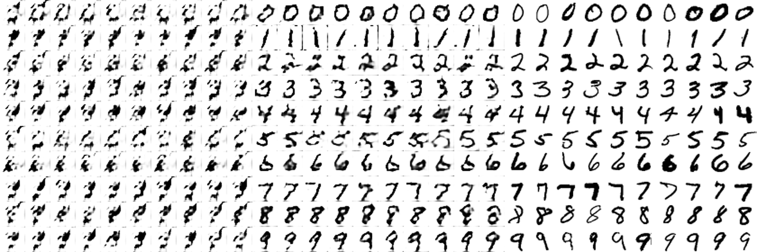
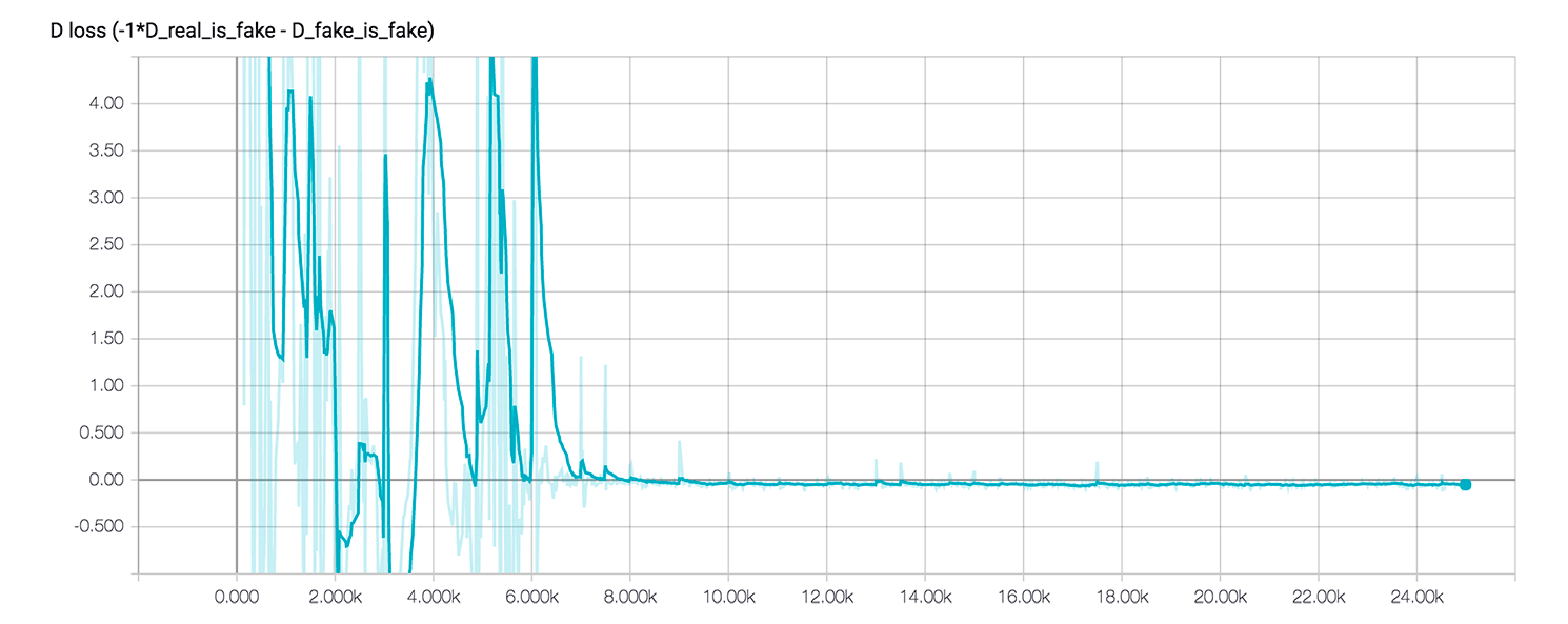
Results

Each second of the video is 250 training iterations. One of the promises of Wasserstein GAN is the correlation between loss and sample quality. As we can see from the loss plot below, after ~8000 training steps loss comes close to zero and indeed, on the video we’re starting to see meaningful images after about 32s.

Wasserstein GAN Loss

Wasserstein GAN in Keras